2577. Minimum Time to Visit a Cell In a Grid

Description

You are given a m x n matrix grid consisting of non-negative integers where grid[row][col] represents the minimum time required to be able to visit the cell (row, col), which means you can visit the cell (row, col) only when the time you visit it is greater than or equal to grid[row][col].

You are standing in the top-left cell of the matrix in the 0th second, and you must move to any adjacent cell in the four directions: up, down, left, and right. Each move you make takes 1 second.

Return the minimum time required in which you can visit the bottom-right cell of the matrix. If you cannot visit the bottom-right cell, then return -1.

 

Example 1:

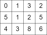
Input: grid = [[0,1,3,2],[5,1,2,5],[4,3,8,6]]
Output: 7
Explanation: One of the paths that we can take is the following:
- at t = 0, we are on the cell (0,0).
- at t = 1, we move to the cell (0,1). It is possible because grid[0][1] <= 1.
- at t = 2, we move to the cell (1,1). It is possible because grid[1][1] <= 2.
- at t = 3, we move to the cell (1,2). It is possible because grid[1][2] <= 3.
- at t = 4, we move to the cell (1,1). It is possible because grid[1][1] <= 4.
- at t = 5, we move to the cell (1,2). It is possible because grid[1][2] <= 5.
- at t = 6, we move to the cell (1,3). It is possible because grid[1][3] <= 6.
- at t = 7, we move to the cell (2,3). It is possible because grid[2][3] <= 7.
The final time is 7. It can be shown that it is the minimum time possible.

Example 2:

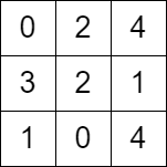
Input: grid = [[0,2,4],[3,2,1],[1,0,4]]
Output: -1
Explanation: There is no path from the top left to the bottom-right cell.

 

Constraints:

• m == grid.length
• n == grid[i].length
• 2 <= m, n <= 1000
• 4 <= m * n <= 105
• 0 <= grid[i][j] <= 105
• grid[0][0] == 0

 

Solutions

Solution 1: Shortest Path + Priority Queue (Min Heap)

We observe that if we cannot move at the cell $(0, 0)$, i.e., $grid[0][1] > 1$ and $grid[1][0] > 1$, then we cannot move at the cell $(0, 0)$ anymore, and we should return $-1$. For other cases, we can move.

Next, we define $dist[i][j]$ to represent the earliest arrival time at $(i, j)$. Initially, $dist[0][0] = 0$, and the $dist$ of other positions are all initialized to $\infty$.

We use a priority queue (min heap) to maintain the cells that can currently move. The elements in the priority queue are $(dist[i][j], i, j)$, i.e., $(dist[i][j], i, j)$ represents the earliest arrival time at $(i, j)$.

Each time we take out the cell $(t, i, j)$ that can arrive the earliest from the priority queue. If $(i, j)$ is $(m - 1, n - 1)$, then we directly return $t$. Otherwise, we traverse the four adjacent cells $(x, y)$ of $(i, j)$, which are up, down, left, and right. If $t + 1 < grid[x][y]$, then the time $nt = grid[x][y] + (grid[x][y] - (t + 1)) \bmod 2$ to move to $(x, y)$. At this time, we can repeatedly move to extend the time to no less than $grid[x][y]$, depending on the parity of the distance between $t + 1$ and $grid[x][y]$. Otherwise, the time $nt = t + 1$ to move to $(x, y)$. If $nt < dist[x][y]$, then we update $dist[x][y] = nt$, and add $(nt, x, y)$ to the priority queue.

The time complexity is $O(m \times n \times \log (m \times n))$, and the space complexity is $O(m \times n)$. Where $m$ and $n$ are the number of rows and columns of the grid, respectively.

Python3JavaC++Go

class Solution:
    def minimumTime(self, grid: List[List[int]]) -> int:
        if grid[0][1] > 1 and grid[1][0] > 1:
            return -1
        m, n = len(grid), len(grid[0])
        dist = [[inf] * n for _ in range(m)]
        dist[0][0] = 0
        q = [(0, 0, 0)]
        dirs = (-1, 0, 1, 0, -1)
        while 1:
            t, i, j = heappop(q)
            if i == m - 1 and j == n - 1:
                return t
            for a, b in pairwise(dirs):
                x, y = i + a, j + b
                if 0 <= x < m and 0 <= y < n:
                    nt = t + 1
                    if nt < grid[x][y]:
                        nt = grid[x][y] + (grid[x][y] - nt) % 2
                    if nt < dist[x][y]:
                        dist[x][y] = nt
                        heappush(q, (nt, x, y))

class Solution {
    public int minimumTime(int[][] grid) {
        if (grid[0][1] > 1 && grid[1][0] > 1) {
            return -1;
        }
        int m = grid.length, n = grid[0].length;
        int[][] dist = new int[m][n];
        for (var e : dist) {
            Arrays.fill(e, 1 << 30);
        }
        dist[0][0] = 0;
        PriorityQueue<int[]> pq = new PriorityQueue<>((a, b) -> a[0] - b[0]);
        pq.offer(new int[] {0, 0, 0});
        int[] dirs = {-1, 0, 1, 0, -1};
        while (true) {
            var p = pq.poll();
            int i = p[1], j = p[2];
            if (i == m - 1 && j == n - 1) {
                return p[0];
            }
            for (int k = 0; k < 4; ++k) {
                int x = i + dirs[k], y = j + dirs[k + 1];
                if (x >= 0 && x < m && y >= 0 && y < n) {
                    int nt = p[0] + 1;
                    if (nt < grid[x][y]) {
                        nt = grid[x][y] + (grid[x][y] - nt) % 2;
                    }
                    if (nt < dist[x][y]) {
                        dist[x][y] = nt;
                        pq.offer(new int[] {nt, x, y});
                    }
                }
            }
        }
    }
}

class Solution {
public:
    int minimumTime(vector<vector<int>>& grid) {
        if (grid[0][1] > 1 && grid[1][0] > 1) {
            return -1;
        }
        int m = grid.size(), n = grid[0].size();
        int dist[m][n];
        memset(dist, 0x3f, sizeof dist);
        dist[0][0] = 0;
        using tii = tuple<int, int, int>;
        priority_queue<tii, vector<tii>, greater<tii>> pq;
        pq.emplace(0, 0, 0);
        int dirs[5] = {-1, 0, 1, 0, -1};
        while (1) {
            auto [t, i, j] = pq.top();
            pq.pop();
            if (i == m - 1 && j == n - 1) {
                return t;
            }
            for (int k = 0; k < 4; ++k) {
                int x = i + dirs[k], y = j + dirs[k + 1];
                if (x >= 0 && x < m && y >= 0 && y < n) {
                    int nt = t + 1;
                    if (nt < grid[x][y]) {
                        nt = grid[x][y] + (grid[x][y] - nt) % 2;
                    }
                    if (nt < dist[x][y]) {
                        dist[x][y] = nt;
                        pq.emplace(nt, x, y);
                    }
                }
            }
        }
    }
};

func minimumTime(grid [][]int) int {
    if grid[0][1] > 1 && grid[1][0] > 1 {
        return -1
    }
    m, n := len(grid), len(grid[0])
    dist := make([][]int, m)
    for i := range dist {
        dist[i] = make([]int, n)
        for j := range dist[i] {
            dist[i][j] = 1 << 30
        }
    }
    dist[0][0] = 0
    pq := hp{}
    heap.Push(&pq, tuple{0, 0, 0})
    dirs := [5]int{-1, 0, 1, 0, -1}
    for {
        p := heap.Pop(&pq).(tuple)
        i, j := p.i, p.j
        if i == m-1 && j == n-1 {
            return p.t
        }
        for k := 0; k < 4; k++ {
            x, y := i+dirs[k], j+dirs[k+1]
            if x >= 0 && x < m && y >= 0 && y < n {
                nt := p.t + 1
                if nt < grid[x][y] {
                    nt = grid[x][y] + (grid[x][y]-nt)%2
                }
                if nt < dist[x][y] {
                    dist[x][y] = nt
                    heap.Push(&pq, tuple{nt, x, y})
                }
            }
        }
    }
}

type tuple struct{ t, i, j int }
type hp []tuple

func (h hp) Len() int           { return len(h) }
func (h hp) Less(i, j int) bool { return h[i].t < h[j].t }
func (h hp) Swap(i, j int)      { h[i], h[j] = h[j], h[i] }
func (h *hp) Push(v any)        { *h = append(*h, v.(tuple)) }
func (h *hp) Pop() any          { a := *h; v := a[len(a)-1]; *h = a[:len(a)-1]; return v }

Comments