3112. Minimum Time to Visit Disappearing Nodes

Description

There is an undirected graph of n nodes. You are given a 2D array edges, where edges[i] = [u_i, v_i, length_i] describes an edge between node u_i and node v_i with a traversal time of length_i units.

Additionally, you are given an array disappear, where disappear[i] denotes the time when the node i disappears from the graph and you won't be able to visit it.

Note that the graph might be disconnected and might contain multiple edges.

Return the array answer, with answer[i] denoting the minimum units of time required to reach node i from node 0. If node i is unreachable from node 0 then answer[i] is -1.

Example 1:

Input: n = 3, edges = [[0,1,2],[1,2,1],[0,2,4]], disappear = [1,1,5]

Output: [0,-1,4]

Explanation:

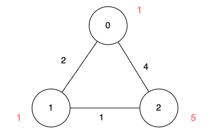
We are starting our journey from node 0, and our goal is to find the minimum time required to reach each node before it disappears.

For node 0, we don't need any time as it is our starting point.
For node 1, we need at least 2 units of time to traverse edges[0]. Unfortunately, it disappears at that moment, so we won't be able to visit it.
For node 2, we need at least 4 units of time to traverse edges[2].

Example 2:

Input: n = 3, edges = [[0,1,2],[1,2,1],[0,2,4]], disappear = [1,3,5]

Output: [0,2,3]

Explanation:

We are starting our journey from node 0, and our goal is to find the minimum time required to reach each node before it disappears.

For node 0, we don't need any time as it is the starting point.
For node 1, we need at least 2 units of time to traverse edges[0].
For node 2, we need at least 3 units of time to traverse edges[0] and edges[1].

Example 3:

Input: n = 2, edges = [[0,1,1]], disappear = [1,1]

Output: [0,-1]

Explanation:

Exactly when we reach node 1, it disappears.

Constraints:

1 <= n <= 5 * 10⁴
0 <= edges.length <= 10⁵
edges[i] == [u_i, v_i, length_i]
0 <= u_i, v_i <= n - 1
1 <= length_i <= 10⁵
disappear.length == n
1 <= disappear[i] <= 10⁵

Solutions

Solution 1: Heap-Optimized Dijkstra

First, we create an adjacency list \(\textit{g}\) to store the edges of the graph. Then, we create an array \(\textit{dist}\) to store the shortest distances from node \(0\) to other nodes. Initialize \(\textit{dist}[0] = 0\), and the distances for the rest of the nodes are initialized to infinity.

Next, we use the Dijkstra algorithm to calculate the shortest distances from node \(0\) to other nodes. The specific steps are as follows:

Create a priority queue \(\textit{pq}\) to store the distances and node numbers. Initially, add node \(0\) to the queue with a distance of \(0\).
Remove a node \(u\) from the queue. If the distance \(du\) of \(u\) is greater than \(\textit{dist}[u]\), it means \(u\) has already been updated, so we skip it directly.
Iterate through all neighbor nodes \(v\) of node \(u\). If \(\textit{dist}[v] > \textit{dist}[u] + w\) and \(\textit{dist}[u] + w < \textit{disappear}[v]\), then update \(\textit{dist}[v] = \textit{dist}[u] + w\) and add node \(v\) to the queue.
Repeat steps 2 and 3 until the queue is empty.

Finally, we iterate through the \(\textit{dist}\) array. If \(\textit{dist}[i] < \textit{disappear}[i]\), then \(\textit{answer}[i] = \textit{dist}[i]\); otherwise, \(\textit{answer}[i] = -1\).

The time complexity is \(O(m \times \log m)\), and the space complexity is \(O(m)\). Here, \(m\) is the number of edges.

Python3JavaC++GoTypeScript

class Solution:
    def minimumTime(
        self, n: int, edges: List[List[int]], disappear: List[int]
    ) -> List[int]:
        g = defaultdict(list)
        for u, v, w in edges:
            g[u].append((v, w))
            g[v].append((u, w))
        dist = [inf] * n
        dist[0] = 0
        pq = [(0, 0)]
        while pq:
            du, u = heappop(pq)
            if du > dist[u]:
                continue
            for v, w in g[u]:
                if dist[v] > dist[u] + w and dist[u] + w < disappear[v]:
                    dist[v] = dist[u] + w
                    heappush(pq, (dist[v], v))
        return [a if a < b else -1 for a, b in zip(dist, disappear)]

class Solution {
    public int[] minimumTime(int n, int[][] edges, int[] disappear) {
        List<int[]>[] g = new List[n];
        Arrays.setAll(g, k -> new ArrayList<>());
        for (var e : edges) {
            int u = e[0], v = e[1], w = e[2];
            g[u].add(new int[] {v, w});
            g[v].add(new int[] {u, w});
        }
        int[] dist = new int[n];
        Arrays.fill(dist, 1 << 30);
        dist[0] = 0;
        PriorityQueue<int[]> pq = new PriorityQueue<>((a, b) -> a[0] - b[0]);
        pq.offer(new int[] {0, 0});
        while (!pq.isEmpty()) {
            var e = pq.poll();
            int du = e[0], u = e[1];
            if (du > dist[u]) {
                continue;
            }
            for (var nxt : g[u]) {
                int v = nxt[0], w = nxt[1];
                if (dist[v] > dist[u] + w && dist[u] + w < disappear[v]) {
                    dist[v] = dist[u] + w;
                    pq.offer(new int[] {dist[v], v});
                }
            }
        }
        int[] ans = new int[n];
        for (int i = 0; i < n; ++i) {
            ans[i] = dist[i] < disappear[i] ? dist[i] : -1;
        }
        return ans;
    }
}

class Solution {
public:
    vector<int> minimumTime(int n, vector<vector<int>>& edges, vector<int>& disappear) {
        vector<vector<pair<int, int>>> g(n);
        for (const auto& e : edges) {
            int u = e[0], v = e[1], w = e[2];
            g[u].push_back({v, w});
            g[v].push_back({u, w});
        }

        vector<int> dist(n, 1 << 30);
        dist[0] = 0;

        using pii = pair<int, int>;
        priority_queue<pii, vector<pii>, greater<pii>> pq;
        pq.push({0, 0});

        while (!pq.empty()) {
            auto [du, u] = pq.top();
            pq.pop();

            if (du > dist[u]) {
                continue;
            }

            for (auto [v, w] : g[u]) {
                if (dist[v] > dist[u] + w && dist[u] + w < disappear[v]) {
                    dist[v] = dist[u] + w;
                    pq.push({dist[v], v});
                }
            }
        }

        vector<int> ans(n);
        for (int i = 0; i < n; ++i) {
            ans[i] = dist[i] < disappear[i] ? dist[i] : -1;
        }

        return ans;
    }
};

func minimumTime(n int, edges [][]int, disappear []int) []int {
    g := make([][]pair, n)
    for _, e := range edges {
        u, v, w := e[0], e[1], e[2]
        g[u] = append(g[u], pair{v, w})
        g[v] = append(g[v], pair{u, w})
    }

    dist := make([]int, n)
    for i := range dist {
        dist[i] = 1 << 30
    }
    dist[0] = 0

    pq := hp{{0, 0}}

    for len(pq) > 0 {
        du, u := pq[0].dis, pq[0].u
        heap.Pop(&pq)

        if du > dist[u] {
            continue
        }

        for _, nxt := range g[u] {
            v, w := nxt.dis, nxt.u
            if dist[v] > dist[u]+w && dist[u]+w < disappear[v] {
                dist[v] = dist[u] + w
                heap.Push(&pq, pair{dist[v], v})
            }
        }
    }

    ans := make([]int, n)
    for i := 0; i < n; i++ {
        if dist[i] < disappear[i] {
            ans[i] = dist[i]
        } else {
            ans[i] = -1
        }
    }

    return ans
}

type pair struct{ dis, u int }
type hp []pair

func (h hp) Len() int           { return len(h) }
func (h hp) Less(i, j int) bool { return h[i].dis < h[j].dis }
func (h hp) Swap(i, j int)      { h[i], h[j] = h[j], h[i] }
func (h *hp) Push(v any)        { *h = append(*h, v.(pair)) }
func (h *hp) Pop() any          { a := *h; v := a[len(a)-1]; *h = a[:len(a)-1]; return v }

function minimumTime(n: number, edges: number[][], disappear: number[]): number[] {
    const g: [number, number][][] = Array.from({ length: n }, () => []);
    for (const [u, v, w] of edges) {
        g[u].push([v, w]);
        g[v].push([u, w]);
    }
    const dist = Array.from({ length: n }, () => Infinity);
    dist[0] = 0;
    const pq = new PriorityQueue({
        compare: (a, b) => (a[0] === b[0] ? a[1] - b[1] : a[0] - b[0]),
    });
    pq.enqueue([0, 0]);
    while (pq.size() > 0) {
        const [du, u] = pq.dequeue()!;
        if (du > dist[u]) {
            continue;
        }
        for (const [v, w] of g[u]) {
            if (dist[v] > dist[u] + w && dist[u] + w < disappear[v]) {
                dist[v] = dist[u] + w;
                pq.enqueue([dist[v], v]);
            }
        }
    }
    return dist.map((a, i) => (a < disappear[i] ? a : -1));
}

3112. Minimum Time to Visit Disappearing Nodes

Description

Solutions

Solution 1: Heap-Optimized Dijkstra

Comments